Beam Hardening Correction (CarouselFit):
Dr. Ronald Fowler STFC Rutherford Appleton Laboratory
Abstract
This document is a brief user guide to the Python software package CarouselFit. This software takes X-ray image data for a number of known samples, and fits them to a model of the beam hardening process which occurs when a broad spectrum source is used to image a sample. This model can then be used to generate corrections appropriate for a single material to convert the observed attenuation values into the actual attenuation that would be observed for that material with monochromatic X-rays at a given energy. This software is based on the IDL package and ideas described in [DEM13].
Introduction
Beam hardening is well known problem that is described in many works, see [DEM13]. Lab based X-ray Computational Tomography (CT) machines use X-ray tubes as their source of radiation. The voltage to the tube can be varied to control the maximum X-ray energy generated, but the actual output is composed of the broad spectrum Bremsstrahlung component and characteristic peaks. The X-ray attenuation of materials (in general) decreases as the energy increases. This means that as a broad spectrum beam passes through a target the low energy X-rays will be absorbed first leaving a beam that has increasing mean energy. It is this effective hardening of the beam that means that a plot of the log of the attenuation against material thickness is not linear, as would be the case if a monochromatic X-ray source was used. Since CT reconstruction algorithms assume that this linear relationship holds artifacts are generated in the final image due to the beam hardening.
To reduce beam hardening artifacts it is usual to pre-filter the X-ray beam with the built-in filters available on CT machines. While this does reduce the problem, it can not fully solve it since filtering to get close to monochromatic beam would leave such a weak high energy beam as to make imaging impractically slow. Hence a compromise has to be made with sufficient filtering to reduce beam hardening effects while allowing enough X-rays through to image the sample in reasonable time. The figure below compares the 80KeV spectra for an X-ray tube with no added filtering and with 1mm Cu filtering. The Cu filter reduces the energy range, but still leaves a polychromatic beam. Plots have been normalised, but the Cu beam will have lower intensity than unfiltered one at all points.
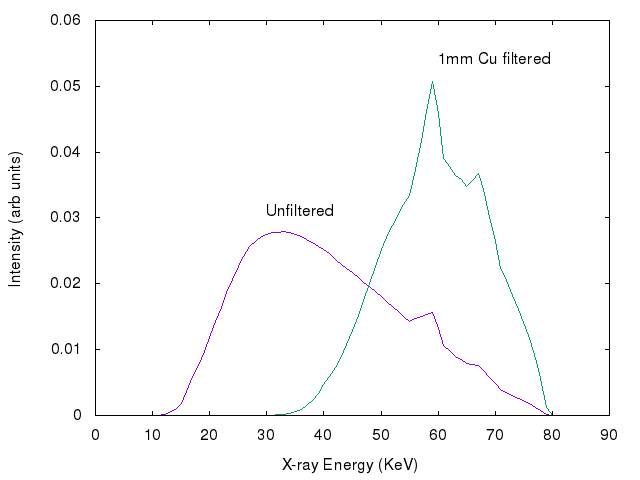
If the energy distribution of the filtered X-ray beam is known, along with the energy dependent attenuation of the sample, then it is possible to apply a correction to the measured attenuation so as to remove beam hardening artifacts. This can be done using the techniques described in [DEM13] which are implemented in this software package.
This software takes as input a number of images of well characterised samples and uses these to fit a simple model of the expected beam hardening (BH) to the observed data. The result is an estimate of the “response function”, R(E), which gives the expected output signal from the detector as a function of X-ray energy for the selected combination of X-ray source, voltage, filters and detector.
Note that due to aging effects of the X-ray source, detector, etc., this function may change over time, so ideally the calibration measurements should be made before and after each CT scan. In addition the model allows for variation in the form of R(E) with the number of the scan line. This can occur due to the way the emitted X-ray spectra is known to depend on the “take-off” angle [DEM13] . Use of pre-filtering the X-ray reduces both beam hardening effects and the variation of these with take-off angle. Low energy X-rays show the greatest variation with take-off angle. Davis recommends using both pre-filtering as well as the software correction described in this guide to best minimise beam hardening artifacts.
Using the fitted response function of the system it is then possible to determine a correction curve that will map from the observed attenuation to the true attenuation that would be seen at a given monochromatic X-ray energy. This correction curve is calculated assuming the sample is composed of a single material type for which the X-ray attenuation coefficient can be determined, using a program such as XCOM [xcom]. This allows for compound materials, as long as the composition is constant. In the case of samples made of more than one compound the correction curve will only be applicable if one material is the dominant absorber and corrections made to that material.
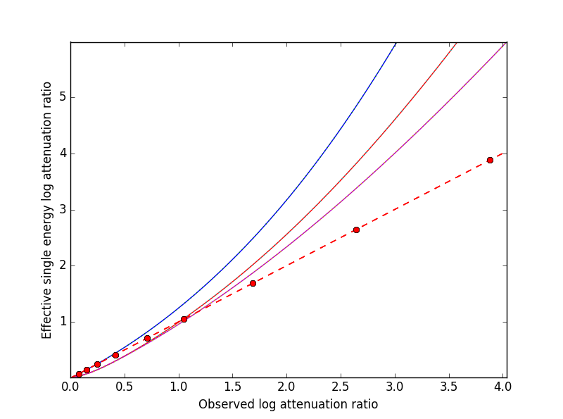
The attenuation correction curve for a material depends on the shape of the energy dependent attenuation within the range of X-ray energies that are present after filtering. If two materials have a near constant ratio of attenuation in this energy range then their correction curves will be similar. However if one has a sharp step in attenuation in this range (a K-edge) while the other does not, then correction curves can be very different. This method is designed for samples of a single material or where one material is the dominant component. The figure below compares the corrections curves for three materials, Ca-hydroxylapatite (brown), aluminium (purple) and tin (blue) with some pre-filtering at 80KeV. The first two have similar correction curves, particularly at low attenuation. The tin curve is different at all attenuations due to a k-edge that causes a jump in its attenuation at about 30KeV.
The next section describes how to download and run the software. The following section describes how to set up the necessary files that give information on the number and type of test images that are used for calibration and the image formats. Details are then given on how to the run the fitting and post-processing image modules of the software. The first of these fits the model to the data while the second applies the correction directly to the CT image data. An alternative to processing all the images is to generates a look-up table or a 4th order polynomial to map observed attenuation values to mono-chromatic attenuation. Such data can be used as input to some reconstuction software, like the standard XTek filtered back projection package and, in future, to the CCPi CGLS iterative code.
Downloading and running the software
Installing the binary
If you have a Python distribution from Continuum(Anaconda https://www.continuum.io/downloads) then you can install the binary package from the CCPi Anaconda channel (https://anaconda.org/ccpi/). To do issue the following at a command prompt:
conda install -c ccpi -c conda-forge ccpi-preprocessing numpy=1.12
This will provide the executables for running the CarouselFit.
CarouselFit
A set of example data to illustrate use the fitting software can be downloaded from the CIL git repository.
Installing from Source
The software is available from the CCPForge repository. It consists of a Python software package along with a number of data files that are used to help model the X-ray beams and the material attenuation. As well as a Python environment the software depends on a number of additional packages being available. An easy way to access most of the required packages is to download the Anaconda Python environment which is available for Linux, MacOS and Windows systems from https://www.continuum.io/downloads. The software has been developed using Python version 2.7, though it should also run with Python 3 as well. It is recommended that the user installs this before installing the CarouselFit software. Alternatively the user may install the required packages in their local Python installation, if they are not already available. The main Python modules that may need to be added to a local installation are:
- numpy - needed for array operations
- matplotlib - needed for plotting
- scipy - needed for optimization
- tifffile - needed for working with tiff images (install from conda-forge channel by: conda -y -c conda-forge tifffile)
The CarouselFit software can be checked out to a suitable directory using the command
svn co https://ccpforge.cse.rl.ac.uk/svn/tomo_bhc/branches/release01 carouselFit
This will create a set of three directories under carouselFit:
- src: this contains the Python source code
- doc: this contains documentation of the software
- test: this contains several sub-directories with information on attenuation and X-ray spectra. The source code must be executed from this directory and any updates to the carousel or crown information should be made in the carouselData sub-directory.
Running a test case
After downloading the software the installation can be checked by running the software in the test directory and reading an example script file.
If the software was obtained from SVN this could be done from a command prompt by typing:
cd test
python ../src/runCarouselFit.py
read script.full
quit
Note that it may be useful to look at the graphs plotted by this process before using the quit command,
since these disappear when the program stops.
If the conda installation method was used then it would be necessary to unzip the test data into a folder. The test data is available from git hub as:
https://github.com/vais-ral/CIL-Docs/raw/master/test/bhctestdata.zip
When this has been downloaded and unziped, get a command prompt in that folder and type the lines:
CarouselFit
read script_demo.txt
quit
This set of commands should run without generating any error messages, such as failure to import modules. If missing modules are reported it will be necessary to add these to the Python system and run the test script again. Check the documentation for your Python system to see how to add modules.
The file script_demo.txt illustrates a simple fitting using some calibration data obtained from QMUL. Lines starting the the # character are comments. The first command in the script loads the files that define the test samples, the imaging voltage and the images themselves. These files, which are explained in more detail later, are:
carousleData/carousel0.def
carouselData/run001.data
carouselData/run001.img
The images that are to used in the calibration are shown by the showimg command. The script then
sets the material and the X-ray energy to be corrected to with the setcormat command.
Then two fits are done, the first allowing for some variation in the fit with the line number in the image.
The second fit does not allow for this variation and assumes that one correction function can be used for
all lines. The final fit returns a 4th order polynomial that can be used to correct the reconstruction of
the image in software such as that used on Xtek machines. The vales of these coefficients are saved in the
file param.log in the same folder that the fitting process was run. For this example data the values should
be:
xpoly:
   0 [ 0.00282561 -0.04733048  0.45413055  0.48893604  0.        ]
The terms in the square brackets correspond to X4,X3,X2,X1,X0 in the input used to an XTek reconsturction.
Configuration files
The original calibration device described in [DEM13] was called a carousel as it was built from a set of 9 test samples arranged between two circular supports allowing for each of the samples to be imaged individually by the scanner. The samples would cover the full range of lines in the scanner, but not the full range of each row; typically only the centre half of each row would be covered by the sample.
A more recent calibration device has been developed at staff at the Research Centre at Harwell (RCaH) which is known as a crown. This device allows a larger number of samples to be mounted. In this case the sample usually covers all lines and rows of the image.
Carousel sample definition file
The materials mounted on the carousel, or crown, must be described in a simple ASCII file which is stored in the test/carouselData directory. An example of the format that was used for the carousel from QMUL is shown below.
# carousel definition file based on data from QMUL 17/11/14
10
Cu,Ti,Ti,Ti,Al,Al,Al,Al,Al,NOTHING
8.92,4.506,4.506,4.506,2.698,2.698,2.698,2.698,2.698,1
0.2093,0.4420,0.2210,0.1105,0.3976,0.1988,0.0994,0.0497,0.02,0.
This illustrates a case where there are 9 sample materials in the carousel. In this case all the samples are pure metals of known thickness and density. It is important to emphasize that the calibration depends on the sample materials been very well characterised. If a large error exists in either the thickness or purity of a sample this can undermine the accuracy of the fitting process. No exact guidelines have yet been defined on the best set of test materials to use, but obviously samples of the material the forms the dominant absorber in the imaged target would be ideal. However, this is often not practical in many cases, such as bone and teeth studies, where calcium metal is the prime absorber, but samples of the pure metal are subject chemical reactions in air. As long as the energy dependence of the sample attenuation coefficient, \(\mu(E)\), is not too different to that of target dominant absorber then the calibration method should work. Some possible problems may occur if the sample has sharp steps in \(\mu(E)\) due to band edges that lie in the response range of the system which are not seen in the target material. For example, compare the attenuation of Sn with that of Ca in the range 0 to 75KeV.
The above file uses the simple format:
- a comment line, starting with #, to describe the file
- a single integer giving the number of sample materials plus 1
- a set of comma separated strings giving the names of each sample, with no spaces. the number of names must be the same as the previous number, with the final one named “NOTHING”. In this case the samples are all pure metals and the chemical symbol has been used as the name. However any name be used as long as a corresponding file with the extension .txt exists in the directory test/xcom. This file gives the energy dependent $mu(E)$ for this sample in steps of 0.5KeV from 0 to the maximum expected energy.
- line4: a set of comma separated values giving the density (in g/cm3) of each sample. A dummy value of 1 is used for the final material.
- line5: a set of comma separated values giving the thickness of each sample in cm. A dummy value of 0. is added on the end.
If a sample type other then the ones already described in texttt{test/xcom} is used it is necessary to create a file of the attenuation values of that sample. See the Readme file in that directory for details.
The thickness range of the samples should aim to cover the range of attenuations that are expected in the test sample.
Sample image data file
In addition to a description of the samples in the carousel it is also necessary to define the format of the sample images and details of the X-ray source, filters and detector. This is done via another file in the directory test/carouselData which has the default extension .data. One such file must be generated for each calibration case, while the above carousel definition file will only change if the samples are changed.
Again a simple ASCII format is used to define the necessary values. An example is shown below:
# data for one QMUL calibration run
80              # voltage
22              # take of angle [not used by default]
W               # target material
19.25           # target density
600             # image res rows
800             # image res lines
carouselData/run001.img         # image file
float32         # data type in image file
2               # number of filters
Al              # filter material
0.12            # filter width
2.698           # filter density
Cu              # filter material
0.1             # filter width - 0.1
8.92            # filter density
CsI             # detector material
0.01            # starting value for detector thickness
4.51            # detector density
The format has one value per line with a comment to described the value. Most of these are self describing, such as the accelerating voltage, the take-off angle, the target material (tungsten, W) and its density, for the X-ray source.
The path to the file containing the sample images must be included in this file. All the images must currently be in a single file. The format used above, float32, assumes a binary format with 9 separate images of \(600 \times 800\) 32bit floating point values. Each value is \(\log ( I_0 / I )\) for that pixel with flat/dark field corrections.
Another supported format is uint16. In this case the sample images values are unsigned 16 bit values of the I value. Again these are all packed in order in a single file. The first image of the file is the (shading corrected) flat field image. The I_0 value is taken as the average of this initial image.
A variation on uint16 format, which is slightly more compact, is labelled as uint64_65535. This format is again unsigned 16 bit images, but it assumes that the data has been corrected for flat and dark fields and that it has been normalised to a white level of 65535. This means that the raw binary file no longer needs an initial image giving the white level. This is the format that is generated by the Python script average_mat.py which converts tif image files into this format. See Appendix A for details of using this program.
Usually a set of filters are used to limit the energy range of the X-ray beam. In the case of the QMUL data they normally employ two filters with 0.12cm of Al and 0.1cm of Cu, as shown in the above file. As the fitting process includes varying the exact Cu filter width it is recommended that a zero width Cu filter element is included even if no Cu was used in the actual imaging.
The definition of the detector material is important and tests to date have been made with CsI. However other materials may be used if their attenuation profile is included in the text/xcom directory. Since the width of the detector maybe used as a fitting parameter it is not essential to specify an accurate value, though this will be used in the command showspec, if it is run before a fit has been performed.
The command line interface
Command list
When the Python software is started from Python or a similar environment, a simple command prompt is issued. Typing help will give a list of the available commands.
The commands are:
- read filename This command opens the given file and reads commands from it until end of file. Control is then returned to the command line. Comment lines start with #. Do not include blank lines in the command script.
- load file.def file.data This reads the definition file for the carousel and the data relating to the actual calibration images. These two files must exist and are described in the previous section. they are normally located in the test/carouselData directory. This is usually the first command to issue since most others need this data to be present.
- quit Exit the program.
- help Give a list of available commands.
- showcor [l1 l2…] This command will plot the attenuation correction curve for any one or more lines. If no arguments are given it will plot the first, middle and last correction lines. The matplotlib zoom feature can be used to focus on a particular region of the plot. It can only be used after a fit has been performed. The correction is shown in the space of log(I0/I).
- showimag This command will plot the images of each sample in one window. It may be useful to check for problems with the samples. It can only be used after data has been loaded.
- fitatt nlines [linestep] This command attempts to fit the model to the selected samples (see mask command). The number of lines of data to fit must be given. This maybe followed by a “step”, e.g. 10 to use every 10th line. This can be useful when using many lines as fitting all of them can be very slow and the fit may not be improved using more data. The time to fit also increases with the number of variables that have been selected with the “vary” command. Fitting to a few lines can be a good way to see if the model fits and give a better initial guess for a fit to a larger subset of the data.
- vary [target|detector|filter|energy|spectra npoly] On its own this command lists the order of polynomial used in fitting the line wise dependence of each of the three main parameters, target width, detector width and filter width. The setting “-1” indicates that the value should be held constant, as set by the initguess command. Using “0” indicates the value will be fitted, but is independent of the line number. Setting to “1” gives a fit allowing a linear variation of the value with line number. For example:
vary filter 0will allow a single fitted value for the filter width.vary detector -1will keep the detector width constant.vary target 1allows the target width to vary linearly with the line number. The fit time increases significantly with the order used and values greater than 1 are not recommended. An experimental option is to allow extra terms to be added to the normally linear dependence of the detector response to the photon energy. Note that energy dependence is NOT related to line number in this case. However this polynomial is not constrained to be positive and the fit may fail. Keeping energy variation off (-1) is recommended. The final option calledspectra, which defaults to 0, i.e. on, when no pre-defined spectra are present, which is the case for the open source release of the package. Setting spectra to 0 causes the calculated spectra to be modelled as a simple non-symmetric Gaussian form with 3 parameters, peak, inverse left width and inverse right width. If pre-computed spectra are available, e.g. from spekCalc, these can be used in preference to the Gaussian by setting vary spectra -1. - initguess [s1 s2 s3 [ s4 s5 s6 s7 ]] Set the initial guess to be used by fitatt. s1 is the width of the target filter (usually tungsten), s2 is the log width of the detector (usually CsI) and s3 is the width of the fitted filter (usually copper). Commonly used values for the initial guess are 0.01 -6.0 0.01. If using the experimental feature “vary spectra 0” than 4 additional values can be given which are the initial value of the energy term (should be zero) plus the Gaussian centre and widths, e.g. 0.01 -6.0 0.01 0.0 40.0 0.05 0.05. When loading data the Gaussian peak is set to half the maximum X-ray energy. Using this command with no parameters gives the current settings on the values.
- mask [n1 n2..] Without arguments this shows the set of masks that control if a given sample will be used in the next fit operation. By default all values are true which means that sample will be used in the fit. Samples are labeled from 1 to n and to mask the m sample that number should be given as an argument to the mask command. A negative value can be used to unmask a previously masked sample.
- setcormat material energy This command must be used before a fit operation to define the material and energy to which the correction curve should be determined. For example setcormat Al 40 sets the correction curve to be calculated for Aluminium at 40KeV. At present if the correction material or energy are altered it is necessary to rerun the fit command.
- transform This is an experimental command which will be removed in future.
- showspec [line] - plot three spectra, the input X-ray spectrum, the filtered spectrum and the response spectrum. Should only be used after a fit has been made. This command needs improving since the “filtered” plot is not meaningful. Also the printed attenuation values are not useful since these are not fitted to. If a line number is given, plots are for that line. The default is line 0.
- showatt [nsamp nline] - plot the sample attenuations along a specific line. By default this shows the attenuation for all samples at line 400. Samples are labeled 0 to $n-1$ in this case.
- debug - set debugging option, for diagnostic purposes only.
- showconf - list some of the settings, such as the filters, detector, source and voltage.
- setwidth [width] - without arguments, prints the width, in pixels, used to average over each line to get the mean attenuation. For the QMUL data, where the sample does not cover the whole image, it is important to ensure this does not exceed the true sample width. For the RCaH data, where the image does cover the whole width, a larger value can be used.
- setfilter [material width] - without arguments lists the filters defined. Can also be used to change the width of existing filters, though not add new ones. Used for debugging.
- setoptions [solver=old|new] - set option. Currently only allows switching between old and new least square solvers in scipy. The old version is more widely available and is the default.
Using the software
Getting the image file
As stated previously it is necessary to write the definition file (.def) that describes the carousel or crown
and the particular test case that is being treated (.data).
The latter file must also point to the data file that contains the sample images in a suitable format.
It is assumed that corrections for dark and flat field images have being applied to the images before they are
passed to the software.
The way in which these are generated will vary with the X-ray CT machine used to gather the images.
For the case of an XTek machine an example python script has been written to illustrate one way in which
suitable calibration data can be obtained from the images of the test samples.
This file is called average_mat.py and can be found in the src directory from the svn checkout.
It can be run from the command line, in a similar manner to the fitting program, though it is not interactive.
It takes a number of arguments, such as:
python ../src/average_mat.py dir_list.txt images.raw
The program requires an input file dir_list.txt which contains an ordered list of directories with
images of the dark and flat field and projections of the samples.
Current practise is to take 11 separate projections of each of the dark field, the flat field and every sample
in the crown. Each file is a 16 bit unsigned image in tiff format. Thus the first directory will have 11 tiff
images of the dark field, and so on.
If there are only three test samples (typically there would be more) then dis_list.txt might be:
c:/Images/crown01/darkfield
c:/Images/crown01/flatfield
c:/Images/crown01/Al0.1
c:/Images/crown01/Al0.5
c:/Images/crown01/Al2.0
Each directory contains a number of tiff images which are averaged over and then used to calculate
the normalised attenuation image for each material sample in the crown. This data is then
written as the raw file images.raw. This can be copied to the carouselData directory and
used as input to a fit run. The first two directories are assumed to be the dark and flat fields
while the rest are the materials in the crown, in this case are aluminium at 0.1mm, 0.2mm
and 0.5mm. The order of the samples in this list must follow the order that is written in the .def
file describing the samples.
The format of the output produced by this script must be given as uint64_65535 in the .data
file.
The average_mat.py script also allows selection of a sub-region of the image. This can be
useful if just doing a fit to a certain region of the image. Four extra parameters can be given
for the minimum and maximum points to output. This reduced image size then needs to be set in the
configurtion file to describe the data.
Running the fitting process
Once the sample image file has been produced and the two data files describing the test samples
and the X-ray conditions written, then the CarouselFit program can be run. This is a
command line program and the user can either type the commands at the prompt or read then from a
previously prepared file.
A simple partial analysis might consist of the following steps which loads the information about the run and displays the images:
load carouselData/carousel0.def carouselData/run001.data
showimg
showatt
When the program reads the image data and the sample descriptions from the files, it performs a basic check to see that the observed attenuation is consistent with the stated voltage and thickness. This helps to catch simple unit errors, or mistakes in the sample order. The following commands can then generate a fit to the supplied sample data:
setcormat CaHydro 40

vary target 0
vary detector -1
vary filter 0

initguess .01 -6 .01
fitatt 800 20

showspec
showcor
These commands then set the material and energy to which we wish to correct the data via the setcormat command, and then alter the default orders of the fit variables. The fitatt command fits the given initial guess across all the lines of the image data (800) but only using every 10th line, which is adequate in most cases. This fit may take around a minute to run. Finally the fitted spectrum and correction curve is plotted. Note that in this case there is no variation of the fit with line number so only a single correction curve will be generated.
The correction curves are stored in the same format as used in the earlier IDL code as separate 8th order polynomial fits to the correction data in a file called polyfit.npz. These curves are the ones shown by the showcor command above. To actually apply the correction to image data requires the use of another Python program, applyTrans.py. In addition to the above 8th order polynomials, 4th order fits are also written to the output file param.log. The 4th order polynomial values are written at the end of the file, one set per line if the solution includes variation with line number. These values can be used in the xtekct file for the parameters X0 to X4, X0 being the rightmost value in param.log. If the variation of the correction with the line number is significant it would be better to correct each project individually as described in the next sectionn.
applyTrans.py
The Python script applyTrans.py can be used to update image files using the correction curves calculated by the above fitting process. It can also calculate a file of type .bht which can be used by XtekCT machines to correct the image data used in CT analysis. In latter case only one correction curve is applied to all the data, in the same way that using the using the 4th order polynomial fit does.
The syntax of the command can be seen using the -h option, which gives:
applyTrans.py [-r rows -l lines -p poly.npz -w whiteLevel -x file.bht]
           [-d] [file1.ext] [filen.ext]
In the above data it is usually necessary to specify the image size in rows and lines. If all the image data is stored in a single file with data type float32, as used for some data from QMUL, then the following command can be used to process it:
python ../src/applyTrans.py -r 600 -l 800 images.raw
In this case the default file polyfit.npz is read to find the correction curves. If 800 curves are present then one will be applied to each line in the image. If only one correction curve is present then this one correction will be used on all image lines. The processed output will be written to bhc_images.raw. Note that the whiteLevel parameter is not needed in this case as the .raw extension is taken to imply float32 data of \(log(I\ :sub:\)/I)`.
To generate a .bht correction file the following command can be used:
python ../src/applyTrans.py -b -x xtekct.bht -w 59200
In this case only the file xtekct.bht is generated. It is necessary to provide an accurate estimate of the white level since any pixels above this are mapped to no attenuation.
References
| [DEM13] | (1, 2, 3, 4, 5) Graham R. Davis, Anthony N.Z. Evershed, and David Mills: Quantitative high contrast X-ray microtomography for dental research: Journal of Dentistry, Volume 41, Issue 5, May 2013, Pages 475–482. |
| [xcom] | M.J. Berger, J.H. Hubbell, S.M. Seltzer, J. Chang, J.S. Coursey, R. Sukumar, D.S. Zucker, and K. Olsen: https://www.nist.gov/pml/xcom-photon-cross-sections-database |